Most database rows describe the present: this customer, this balance, this order. Time-series data describes the past on its way to becoming history — meter readings, request latencies, machine vibrations — arriving constantly, queried by recency and window, rarely updated and almost never deleted one row at a time. That asymmetry shapes everything about how it should be stored.
What makes time different
Three properties separate time-ordered workloads from ordinary transactional ones. First, arrival order is roughly time order: the common case is append, which means the storage layout can assume recency clusters together. Second, queries are windows, not points: the last hour, this shift versus last shift — predicates over ranges of time, not single keys. Third, old data cools into aggregates: raw points matter for days, hourly rollups matter for months.
A general-purpose row store can serve all three, but only if the engine knows time is special: indexes on the timestamp, pruning that skips whole regions without reading them, and encodings that exploit the fact that consecutive timestamps differ by small, regular amounts.
A realistic telemetry example
Consider press-line meters reporting every minute. One row per event, a TIMESTAMPTZ column carrying the time, volatile dimensions in a JSON payload:
CREATE TABLE readings (
  device  text,
  ts      timestamptz,
  payload jsonb
);
CREATE INDEX readings_ts ON readings (ts);
One event looks like this on the wire — flat time and device columns, volatile dimensions in the payload:
{
  "device": "press-07",
  "ts": "2026-09-25T08:14:00Z",
  "payload": { "kwh": 41.7, "line": "B", "shift": "morning" }
}
SELECT device, avg((payload ->> 'kwh')::float) AS avg_kwh
FROM readings
WHERE ts > now() - INTERVAL '8 hours'
GROUP BY device;The ts predicate does the heavy work: it prunes storage to the recent slice before any row is examined, and the per-device grouping runs over that slice only. The same payload pattern from Bringing SQL and JSON Workloads Together carries the dimensions, so no second system is needed for the flexible half.
How the storage earns it
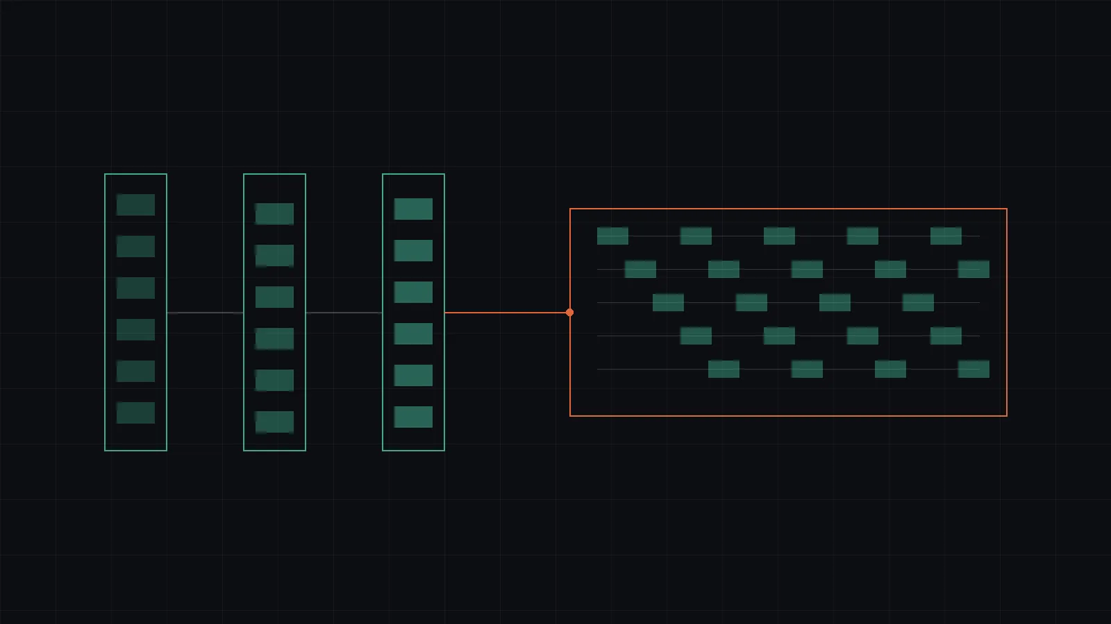
Underneath, two mechanisms do the real work. Timestamps flush into columnar runs encoded as deltas — consecutive readings differ by a minute, not by an epoch — and sorted keys compress by run length. Scans then prune through a metadata pipeline: zone maps, BRIN ranges, probabilistic filters, and bitmap indexes, falling back to exact checks only where the metadata cannot prove a miss.
The honest boundary: there is no dedicated time-series engine in the current version — no hypertables, no continuous aggregates, no retention policies, no downsampling. Time series today means temporal columns plus SQL plus ts indexes plus columnar pruning, documented under the time-series guides. Anything beyond that is roadmap, and the roadmap says so.
An industrial reading
On a factory floor, the query that matters is rarely exotic: which press drew more than its shift baseline in the last hour? That is a windowed aggregate over recent rows, grouped by device, filtered by a threshold — the exact shape above. Because history sits next to current state in the same layer, the follow-up question (and what work orders were open on those presses?) is a join, not an export. One copy of the truth is the whole point of the unified data layer.
Time moves one way. Storage that respects that — append-friendly, window-queryable, pruned before it is read — turns telemetry from a pipeline problem back into a query.